
 All articles
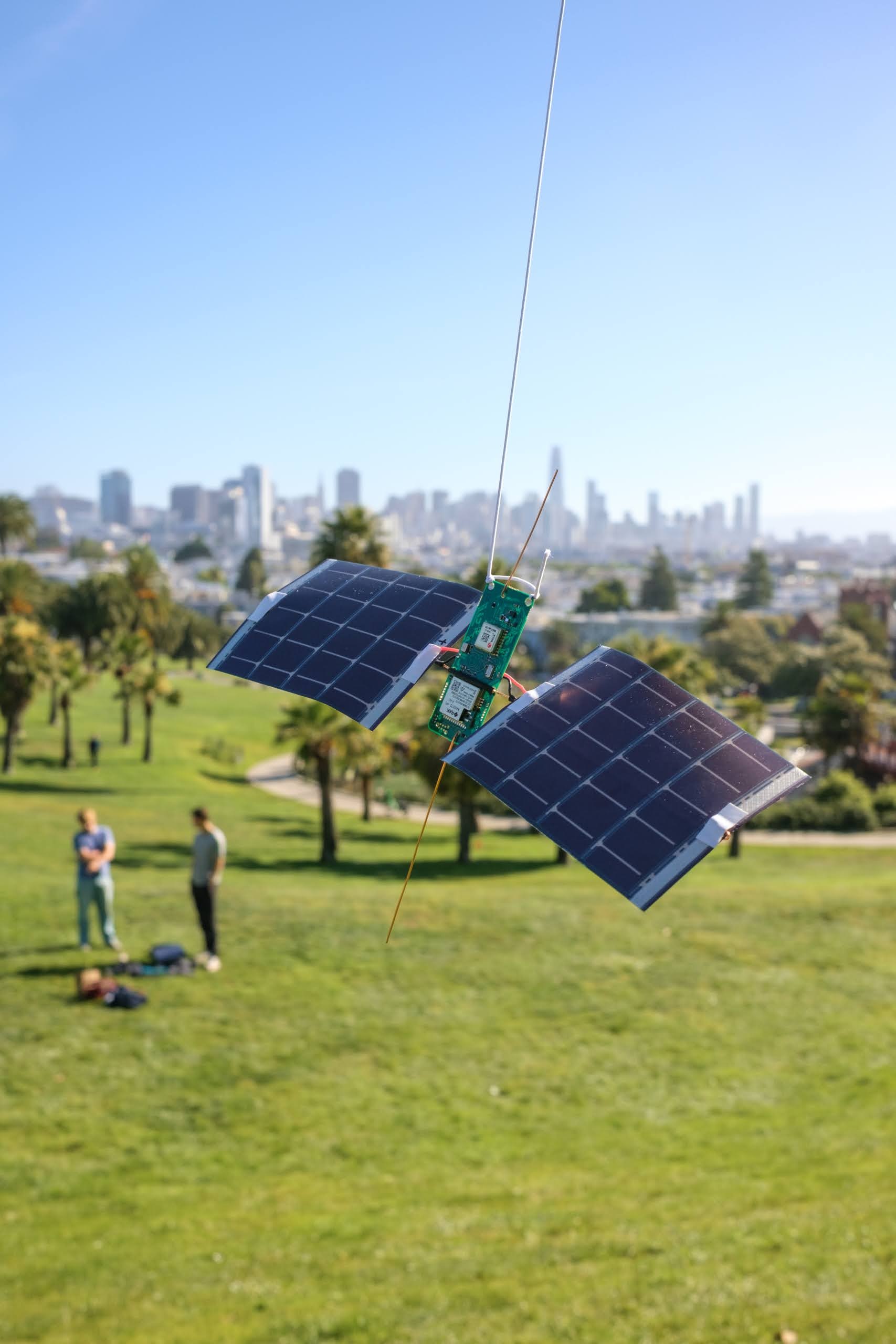
I’ve spent a lot of time between launches modeling the antennas, testing the firmware, and measuring where the power goes. Some changes made substantial differences. This is a dev log of that work.
The board
Caleb Kruse, Shepherd Kruse, and I launched Stratolink 3 in May 2026. It was our first flight; the numbers identify individual payloads. By then the board had most of the hardware I wanted, though the firmware was still pretty minimal: get a GPS fix, read the sensors, send a packet, and go back to sleep.
I’ve been working toward v1 on the other two payloads, Stratolink 2 and Stratolink 1. That means using the rest of the hardware and making sure the board recovers when the capacitor runs out.
The board is about 23.4 by 57.3 mm, made from 0.4 mm FR4. The RAK3172 contains our STM32WL processor and LoRa radio, the u-blox MAX-M10S handles satellite positioning (GNSS), and the BQ25570 charges the capacitor from the solar panels. Around those are the sensors for pressure, temperature, UV, light, acceleration, and sound.
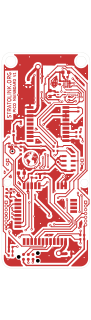
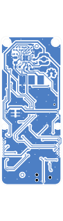
The one we flew in May weighed 10.28 g without its string; by July I had the next assembly down to 9.62 g. Those are assembled weights, including the solder, panel supports, wire, and glue.
Wire antennas
I started with quarter-wave monopoles: short pieces of wire we can cut to length and solder straight to the board. Divide the speed of light by four times the frequency to get a starting length:
That gives us 81.9 mm at 915 MHz, 86.3 mm at 868 MHz, and 47.6 mm for GPS L1 at 1575.42 MHz. Our US flight packets were actually around 904–905 MHz, so for those channels we’re closer to 83 mm.
The two solar panels complicate this. Their conductive material affects the antenna, along with the board, feed, and wire coating. I modeled the monopole alongside vertical and horizontal dipoles, plus a crossed-dipole arrangement. A dipole gives us a second arm of a known length; with the monopole, the rest of the payload becomes part of what we’re trying to tune.
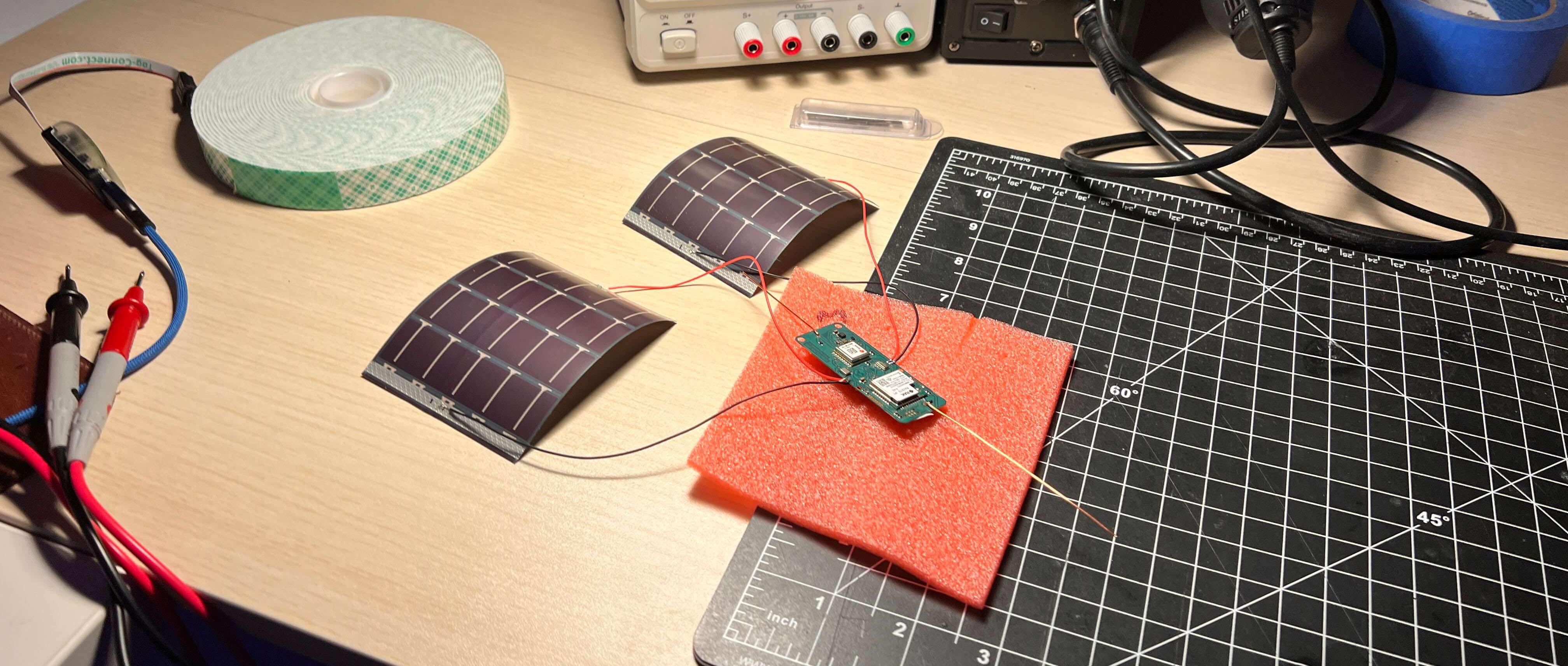
We used copper wire, though Shepherd also suggested guitar string. I was interested in how well the wire would hold its shape. There isn’t much point getting the length right if it bends against a solar panel while we’re assembling everything.
Temperature and wire length
I also checked how much the copper would shrink in the cold. Cooling an 86.2 mm element from 20°C to -50°C shortened it by about 0.10 mm and moved the modeled resonance by less than 1 MHz. That’s small relative to the matching bandwidth in this model.
The enamel was harder to account for. I tried a dielectric-loading estimate, but it was too rough to turn into a reliable correction to the cutting length. I still want to put the complete assembly on a network analyzer, with the actual wire and panels fitted.
Including the solar panels
I got the geometry wrong in my first pass. I’d left out the panels and oriented the simplified PCB ground incorrectly, which made the monopole look poorly matched and a separate dipole look much more attractive. So I rebuilt the model around how the payload actually hangs.
With that fixed, I could toggle the panels on and off and compare. Even with no electrical connection to ground, they changed the radiation pattern quite a bit. The impedance match was actually slightly better without them, but I was also interested in how much signal went toward the ground stations. Below are two vertical cuts through that pattern at 904.5 MHz.
At float altitude, a ground station a hundred kilometers away is only a few degrees below the balloon’s horizon. A vertical wire sends most of its radiation out to the sides, with a weak spot along the wire itself. The full pattern looks like this:
To work out which parts of the pattern mattered, I went back through our received packets. This turned up a fairly annoying GPS bug. After the GNSS module stopped getting fresh fixes, the firmware could keep sending its last valid coordinates. The radio was still working, but the position inside the packet was old. Filtering those out brought the longest apparent link down from 433 km to about 252 km.
That left 50 receptions with a distinct balloon fix and a known ground-station position. The median receiver sat about nine degrees below the horizon. I used those directions to weight the antenna comparisons, so I was comparing gain toward places we’d actually received a packet.
I also moved the panel’s ground connection closer to the antenna feed in the model. I figured a shorter bond wire would help, but with the antenna length held fixed it made the match worse. Tuning the wire for each arrangement recovered most of that loss, without giving me much reason to prefer the shorter connection.
Antenna model assumptions
I used NEC antenna-modeling software for these calculations, representing the panels as flat conductive grids roughly 70 by 100 mm, with dimensions estimated from the assembly photo. The PCB ground, panel substrate, flex, wiring, and power circuitry are all simplified. I wouldn’t choose between real assemblies on a few tenths of a decibel from this model alone.
The flight sample is small too. Filtering for distinct coordinates removes the repeated fixes, but it doesn’t independently verify every remaining position.
Hang angle and suspension
We’d hung the first payload from a corner, so the whole assembly leaned to one side. Before changing the suspension, I wanted to see how much reception we were giving up by leaving it that way.
I pulled 177 accelerometer samples from after Stratolink 3 had reached float altitude. The board’s y-axis stayed fairly close to 20 degrees from gravity in those samples. There are minutes between readings, so I can’t reconstruct all the swinging in between, but I had an angle to start with.
Using the same receiver directions as before, I tilted the antenna model and averaged its gain over a full turn. I had to assume it spent equal time facing each direction, since the accelerometer can’t tell me its yaw.
Straightening it helped a little. With the panels included, a 20-degree lean only cost the monopole about 0.08 dB. Even at 45 degrees, the loss stayed below half a decibel. The vertical dipole was more sensitive to the same tilt.
My suggestion was to use two attachment points, with the lines meeting above the center of mass. That should let us straighten the board without adding much weight. Given how small the modeled improvement was, I didn’t see a reason to build anything more involved.
We also went back and forth on the string. I wanted less stretch so the payload wouldn’t bounce as much; Caleb liked how securely the stretchy line cinched. I had some kitchen twine ready before Stratolink 2’s launch in July and we planned to bring both. I haven’t done a controlled comparison of the two.
Moving to SF9
Changing the radio settings made a larger difference in the model. LoRa encodes symbols as frequency sweeps, or chirps. Increasing the spreading factor stretches each chirp out in time, giving the receiver longer to pick it out of the noise. I used a roughly 5 dB sensitivity improvement from SF7 to SF9 in the link-budget model. You can see how the chirps change below.
The longer chirps cost airtime. Our original 35-byte telemetry payload took about 98 ms at SF7 and 308 ms at SF9, including 13 bytes for LoRaWAN, the networking protocol we use. Keep sending every five minutes and we’d be on air for almost 89 seconds a day.
Our packets reach the internet through ground-station gateways on The Things Network (TTN). Its public Sandbox gives each device 30 seconds of uplink airtime per day, so I needed to space the packets out. My first suggestion was fifteen minutes, which used nearly all of that allowance. We settled on twenty minutes when the board has enough stored energy to run its full schedule, leaving room for other uplinks.1
The telemetry format later grew to 40 bytes. At SF9 the larger packet takes about 329 ms, totaling 23.7 seconds a day at twenty-minute intervals. Fifteen minutes would already put us over 30 seconds, even before any other uplinks.
I left the board running overnight at SF9 and it kept cycling and sending. Comparing reception in flight will take more data, especially after the stale GPS fixes in the first run.
Airtime assumptions
The calculation uses an explicit header, CRC, eight-symbol preamble, and coding rate 4/5. The packet also includes the encoded payload symbols. Low-data-rate optimization is enabled at SF11 and SF12. Those two rates are shown for comparison; they are not standard US915 uplink settings. TTN’s usage policy and regional radio rules are separate constraints.
The 5 dB difference is the receiver-sensitivity assumption I used in the model. I haven’t measured that improvement across our receiving gateways.
Sharing the radio
With twenty minutes between telemetry packets, we have a radio sitting idle for most of the cycle. I wanted to use that time to relay messages for Meshtastic, an open-source LoRa messaging system.
We only have one radio, so this means switching the STM32WL between the two configurations. It has to finish the LoRaWAN receive windows before listening for Meshtastic traffic, then switch back for the next telemetry packet. I also need to limit the relay’s energy use and airtime so it doesn’t use up what we need for tracking.
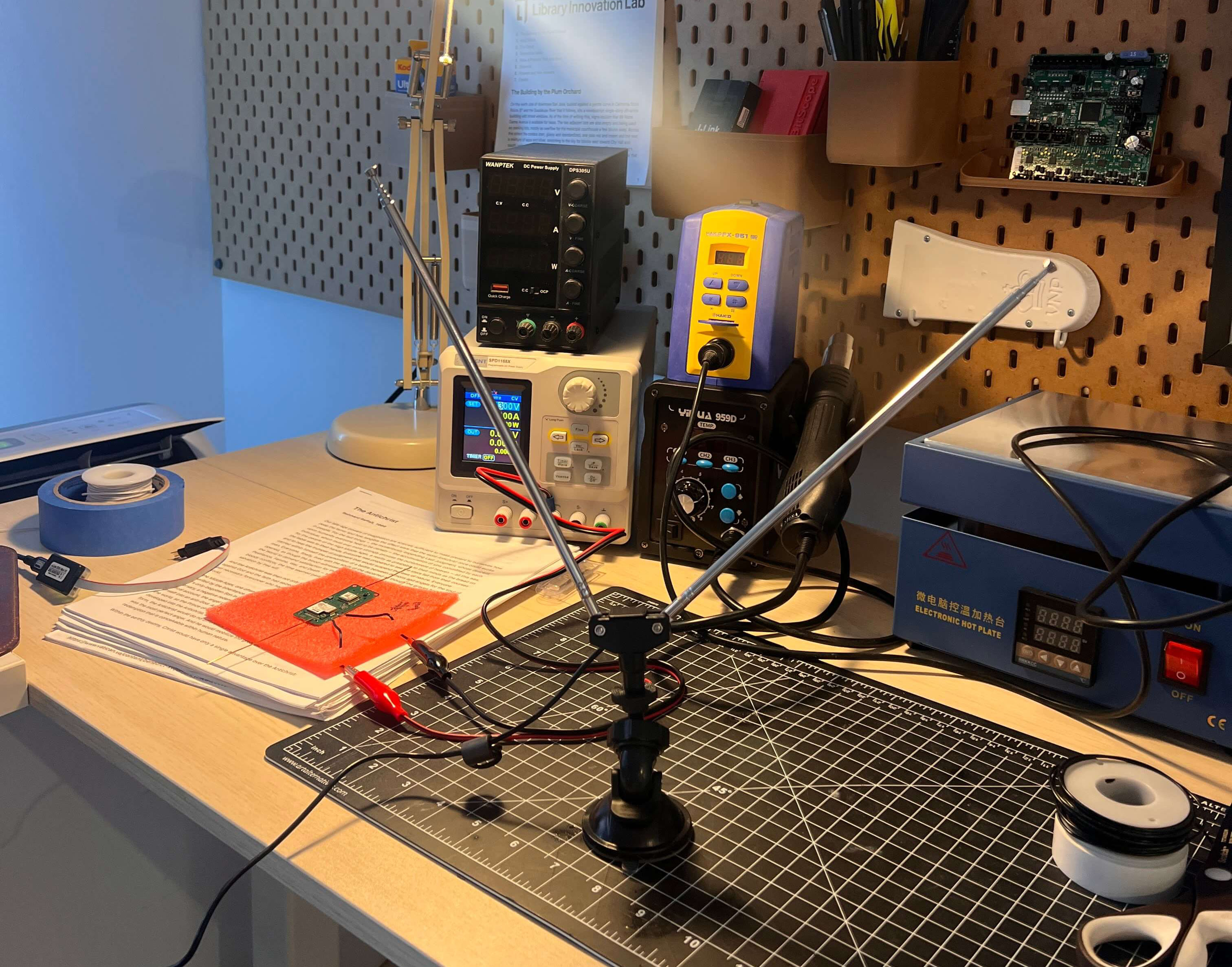
By June 3 I had the board receiving local Meshtastic traffic using its LongFast radio preset between TTN transmissions. My roommate and I sent messages back and forth while I watched on a software-defined radio (SDR). Below is a capture across both bands, followed by a closer look at the individual chirps. The narrow bursts are our SF9 telemetry; the wider ones are SF11 LongFast.
I added counters to keep track of packets received and forwarded, along with duplicates and packets that had reached their forwarding limit. Over an 18.3-hour bench run, the board received 2,215 packets and forwarded 1,412, while continuing to send its own telemetry.
I was powering that run from the bench supply, so I still need to repeat it on solar power. Keeping the radio listening is a significant addition to the power budget.
Reading the waterfall
Frequency runs left to right and time runs downward. The color is relative FFT power, rather than calibrated dBm. There’s also a thin line at the capture center, where the SDR can introduce its own DC artifact. Some of the other signals belong to nearby radios.
For the wide view, I kept the peak within each displayed bin so short bursts wouldn’t disappear. The close views select roughly 55 ms around a strong burst from the saved IQ samples and center its frequency.
The relay plot counts the board’s receives and forwards. It doesn’t establish how many of those forwards reached another receiver.
The supercapacitor
I went with solar panels and a supercapacitor to keep the weight down. Acquiring a GPS fix and transmitting uses enough of that stored energy that the board needs to spend most of the time between packets asleep.
The capacitor we fitted is a DMF4B5R5G105M3DTA0, rated at 1 F and 5.5 V and weighing about 1.3 g. I cared about its resistance as well as its capacity. This one has a typical equivalent series resistance of 40 milliohms at 1 kHz; some similarly sized capacitors meant for clock backup have far too much resistance to supply a radio burst.2
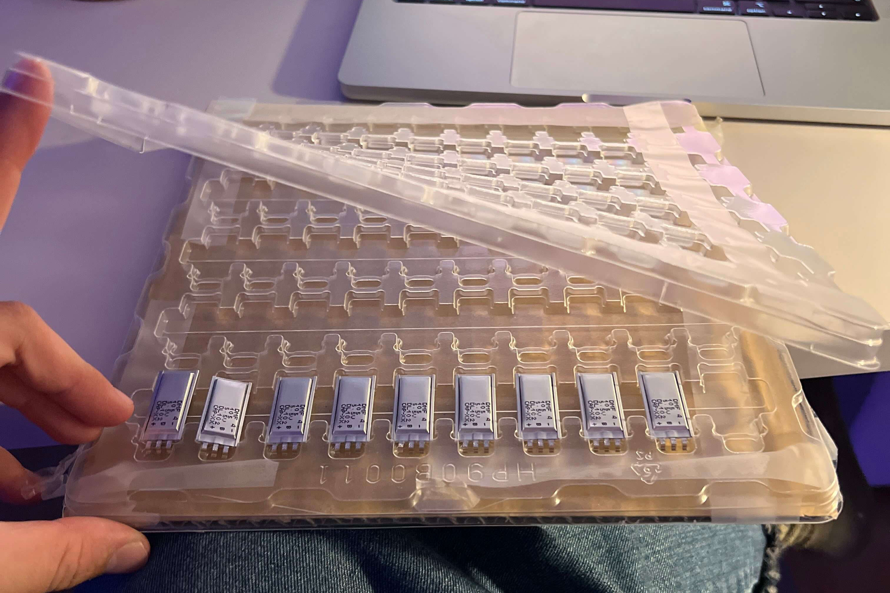
At 120 mA, 40 milliohms would give an immediate drop of just 4.8 mV in a simple series-resistance model. Then the voltage keeps falling as the burst removes charge. To estimate the energy we have available, we can use:
A 1 F capacitor charged to 5 V stores 12.5 joules. Let it fall to 3.32 V and we’ve used about seven joules, before conversion losses. I’m using 3.32 V as a common endpoint for the calculations below, not as the board’s shutdown voltage. An earlier version of the firmware’s voltage conversion could flatten the reported reading around there, so I can’t use that plateau to tell when the capacitor was actually empty.

I initially tried charging the first capacitor under a lamp, which took long enough that I fell asleep waiting for it. After that I charged it from the bench supply so I could work on the firmware without waiting on the light source. In May I found that the GPS task kept running even when the firmware switched to a reduced-power schedule. Once I fixed that, the board could finally go quiet at night and cold-start again in the morning.
Sleep current
In one of the earlier overnight runs, current settled around 33–35 µA. The J-Link debugger I use to inspect the running firmware was still attached, so I’m keeping that separate from the flight power budget. There are quite a few things drawing current besides the sleeping processor: dividers, regulators, sensors, leakage, and potentially the debugger.
To see how little margin we have, take a constant 40 µA load. An ideal 1 F capacitor drops from 5 V to 3.32 V in about 11.7 hours. Use the part’s minimum rated capacitance of 0.8 F and that falls to 9.3 hours, without waking the GPS or radio once.
The voltage-divider resistors use some of that budget too. A 1 MΩ / 1 MΩ divider draws 2.5 µA at 5 V, while a 100 kΩ / 100 kΩ pair draws 25 µA. Higher resistance helps, provided I give the analog-to-digital converter’s input enough time to settle before reading it.
I also need to test the assembled board in the cold. The May flight reported a board temperature of -42.1°C, just below the capacitor’s -40°C rating. Receiving a packet at that temperature doesn’t tell me how well the capacitor will charge and discharge through repeated cold cycles.
Charge limits and capacitor measurements
The datasheet’s AC resistance is useful for comparing parts, but I still need to measure the fitted capacitor’s response to a radio burst, including at low temperatures.
The charge ceiling needs room for resistor tolerance too. This capacitor contains two cells and has a midpoint terminal, so reading the total voltage won’t tell me whether one cell is over its limit. Any current used to balance them also comes out of the overnight budget.
Choosing the measurements
We spent a lot of time going through things we could measure from a balloon. Pressure and temperature were the obvious ones, but we also talked about ozone, aircraft acoustics, tracking radio-tagged animals, and measuring the atmosphere along the radio path itself. Some needed another sensor; others came down to what we could do with the radio and processing time we already had.
Pressure and temperature
The MS5611’s pressure range goes down to 10 mbar, which helped me choose it over environmental sensors that stop well above the pressures we’re interested in. It lets us follow the pressure change during ascent and compare that with GPS altitude, using temperature and an atmospheric model to relate the two.3
Getting the units right took me an extra attempt. After applying the sensor’s compensation (including the correction for low temperatures), I multiplied the pressure by ten where I should have divided by ten. The value overflowed our sixteen-bit telemetry field before it even left the board.
For a separate temperature reading I used a TMP117 on the existing I²C bus. It tells us the temperature at the board, where sunlight and heat from the electronics affect the reading. Before using it as an air-temperature measurement, I need to characterize those effects and the mounting.
UV and ozone
I was particularly interested in whether we could infer ozone from optical measurements. Ozone absorbs some UV wavelengths more strongly than others, so measuring that absorption as the balloon rises could tell us about the ozone above it without carrying a chemical sensor.
I looked at the AS7341 for visible and near-infrared spectral measurements too, but it needed a separate 1.8 V supply. For this board I went with the LTR390, which gives us UV and ambient light on the 3.3 V rail we already have. Its UV output is one broadband channel, though. To compare separate UV bands we’d need different hardware.4
Turning those counts into an ozone estimate will take calibration. Clouds, the sun’s angle, and the payload tilting all change the light reaching the sensor. I need to keep the gain and integration time with the raw counts, work out the orientation, and calibrate the optical response. A second UV band would help distinguish changes in absorption from a change in how brightly the sensor is lit.
From UV to an ozone estimate
For direct sunlight, we can start by integrating the incoming spectrum over the detector’s response:
R is the sensor response, σ the wavelength-dependent ozone absorption cross-section, and N the ozone column along the light path. To use this on flight data I’d also need to account for cloud scattering and the detector’s angular response. I haven’t recovered a validated ozone profile from this flight.
The spectral cross-sections are measured data available from Serdyuchenko and colleagues.
Motion and acoustic sensing
The LIS2DH12 accelerometer supplied the mounting-angle data from earlier. It can also wake the processor when it detects selected motion events, which saves us polling it continuously.
I added the T3902 microphone to try detecting acoustic events on the board. On the first flight we only sent back a single bit when it triggered. That bit fired much more often than I expected, and the rate varied with daylight. I suspected switching noise from the solar harvester, though temperature was changing at the same time.
One event bit wasn’t much to debug from, so I used J-Link to capture the microphone’s raw output: a fast stream of ones and zeros called pulse-density modulation (PDM). Even in a quiet recording, the proportion of ones wasn’t exactly 50%. Our decoder subtracted a fixed midpoint, leaving a DC offset that the event detector counted as sound. Below are two decodes of the same recorded 1 kHz tone.
Calculating variance removed the DC contribution. In the saved tone and silence recordings, that took the tone-to-silence ratio from about 28:1 to 233:1. I also tried a better anti-alias filter offline, which lowered the spectral floor. The variance fix could go into the event detector without bringing that whole filtering pipeline into the flight firmware.
On the bench, I got a useful response from roughly 200 Hz to 4 kHz. Measuring infrasound, below the range of human hearing, would need another transducer. With this microphone I’m interested in small features we can calculate on the board and fit into a packet, since there’s no room for continuous audio over this link.
Position, timing, and the radio path
We also discussed measuring the atmosphere along the path from a balloon to a ground station. I worked through the position and timing precision we’d need for that.
For the measurements taken on the board, I mainly need to know where and when each sample was collected. Add a position uncertainty and sensor calibration, and we can start comparing those samples with a weather model. The low-power MAX-M10S is a standard-precision receiver and suits that tracking job. Getting it to return a fresh fix was more pressing than improving its nominal accuracy.
Measuring the radio path is much harder. We’d be trying to separate a small atmospheric delay from the time the signal takes to cross the geometric distance, plus the offsets in our clocks and the delays inside both radios:
Ten nanoseconds of timing error looks like about three meters of extra path. A hundred nanoseconds looks like thirty meters. To resolve 30 cm, we’d need roughly a nanosecond of combined timing precision and endpoint positions accurate enough to match. A GPS timestamp attached to a packet doesn’t get us there.
For that experiment I’d need timestamps tied to the actual RF event, then measurements of the clock offsets and hardware delays. By the time a packet reaches our server, network transport and processing have added their own delays. Our current telemetry can’t separate those out.
We do get signal strength from the receivers. Using that to say something about the atmosphere means accounting for distance, transmit power, the ground station, and how the payload is oriented. Some of the apparent atmospheric variation would just be the balloon turning, which is another reason to characterize the antenna and hang angle.
Receiver requirements
The MAX-M10 family has a time-pulse output, but I still need to account for its jitter, how the processor captures it, the RF timestamp, antenna and cable delays, and position errors at both ends. GNSS carrier-phase sounding would need another set of receiver capabilities. I haven’t settled on an upgrade for either approach or recovered an atmospheric measurement from the radio path.
Coverage in moving air
Below is a render made by Caleb that follows 30 balloons over 14 days. I wanted to get a sense of how much ground we could cover with more of these in the air, and how the wind would spread them out or bunch them together.
The interactive version uses Caleb’s trajectory code with historical winds from NOAA’s NCEP/DOE Reanalysis 2 at 300 hPa, covering May 17–31, 2024. We can start the fleet in either hemisphere or split it between both. Adding balloons keeps the existing tracks in place.
Each circle is an assumed radio footprint. The percentages count how much area falls inside at least one circle at that moment, with separate totals for each hemisphere and Earth.
Wind simulation assumptions
Caleb’s solver advances hourly, using the nearest wind-grid point and interpolating between six-hour wind fields. Each balloon stays on the 300 hPa pressure surface and follows the horizontal wind. These are historical winds, not a forecast or a reconstruction of Stratolink 3.
The northern and southern fleets each have 500 starting positions sampled uniformly by area with separate fixed random seeds. The worldwide fleet alternates between the two sets, so 500 balloons means 250 in each hemisphere. Every balloon is already afloat at the start. These positions are a way to compare distributions, not proposed launch sites.
We count coverage at 6,000 equal-area points, using the hourly track samples. The circles assume the same range in every direction. Terrain, power, collisions, link margin, ascent, and balloon failures are left out.
Source: NOAA Physical Sciences Laboratory, NCEP/DOE Reanalysis 2. Coastlines are from Natural Earth.
Waiting for a contact
Caleb pointed out that a remote sensor probably doesn’t need a balloon overhead all the time. It might be fine waiting a day, or a few days, to send its measurements. The coverage circles move, so looking at one frame misses a lot of the area the fleet eventually reaches.
To check that, we can keep a record of when each location falls inside a footprint. There are two useful counts here: the area reached at least once, and how long a message waits for the next visit. A location reached on the first morning can still be left waiting for the rest of the week.
With 500 balloons split across both hemispheres and a 350 km radius, this run starts with about 31% of Earth inside a footprint. By the end of the first week, about 99% has been reached at least once. That’s a much larger area, though a single visit only helps if the sensor is ready to transmit when the balloon passes.
For the waiting-time calculation, we give each location a message at every hourly sample during the first week and look ahead for up to seven days. About 71% of those messages find a geometric contact within a day; about 98% within a week. At 100 balloons, those figures fall to about 25% and 72%.
| Balloons | Area visited in week 1 | Messages with contact within 1 day | Within 7 days |
|---|---|---|---|
| 30 | 40% | 9% | 39% |
| 100 | 71% | 25% | 72% |
| 500 | 99% | 71% | 98% |
At a 250 km radius, closer to the longest reception we can substantiate from our flight, 500 balloons give about 57% of messages a contact within a day and 94% within a week. The assumed range matters even with this many balloons.
I’m more interested in whether we can keep returning to the same places. In the 500-balloon run, about 92% of Earth gets an opportunity within seven days of every sampled arrival. That drops to 48% at 100 balloons. The map lets us inspect individual locations, since the global average hides the places that keep getting missed.
Starting all 500 in the north changes the result substantially: almost the entire northern hemisphere gets a visit in week one, but only about 19% of the south does. Some tracks cross the equator during the run; that doesn’t make a northern fleet a substitute for launching in both hemispheres.
Counting waits and repeat contacts
For a location x and a message ready at hour t, we find the first later sample within the chosen radius of any balloon. A message ready while a balloon is already in range has zero wait. All hourly arrivals from hour 0 through 167 have a full 168-hour look-ahead available in the saved tracks.
The deadline curves count every arrival, including ones that never find a contact. A week-long wait at an unreachable location must not disappear from the average. The displayed mean caps each wait at seven days:
This is a restricted mean, not an estimate of the full waiting time. If a message still has no contact after seven days, we only know that its wait exceeds that window. Medians and 90th percentiles beyond it appear as “>7 days.” The seven-day repeat-contact figure counts locations where every sampled arrival meets the deadline.
Area results weight the 6,000 points equally. Message results also weight the 168 arrival times equally. Selecting a point on the map calculates its contacts directly from the tracks, rather than borrowing the nearest sampled location’s result.
For the 500-balloon worldwide case, increasing the area sample to 24,000 points changed the one-day, seven-day, and repeat-contact percentages by less than 0.2 percentage points. Sampling along the same tracks every fifteen minutes changed the capped mean wait from 24.0 to 23.7 hours. These checks concern sampling resolution, not the accuracy of the wind trajectories.
Contacts are sampled hourly, so the model can miss a brief pass or place a boundary up to a sample apart. We don’t loop the end of the weather record back to the start when calculating waits. The animation loops only for playback.
We still have to get a packet through. The surface sensor and balloon need to be awake, on compatible settings, and have enough link margin during the pass. Getting the packet back to us adds another wait if there’s no gateway nearby. Storing it on the balloon would let it carry the data to a receiver later, but this simulation doesn’t model that second leg.
These two weeks give us a useful comparison between fleet sizes. Before choosing a number to deploy, I’d want to repeat it across seasons and pressure levels, use actual launch sites, and include night-time power loss and failed balloons. Then we can choose a deadline for a sensor and see how often we meet it.
Snapshot coverage
There’s also a simpler calculation we can use to check the starting coverage. Place balloons independently across Earth, give each the same radius, and count overlapping circles only once:
With a 350 km radius, 100 active balloons cover an expected 7.3% of Earth. At 500 we get 31.4%, and at 1,000 we get 53.0%. Going from 50% to 75% takes roughly twice as many balloons because more of the added area overlaps places we already cover.
| Coverage | 250 km | 350 km | 400 km |
|---|---|---|---|
| 25% | 748 | 382 | 292 |
| 50% | 1,801 | 919 | 704 |
| 75% | 3,601 | 1,838 | 1,407 |
| 90% | 5,982 | 3,052 | 2,337 |
The radius changes those counts substantially. At ten kilometers altitude, the geometric horizon to sea level is about 357 km, or about 412 km with a common atmospheric-refraction approximation. Our filtered flight data gives us a reception at about 252 km. I can use the larger radii to explore fleet sizes, but we haven’t demonstrated reception all the way out to those horizons, or in every direction.
Coverage calculation
For Earth radius R and surface footprint radius r, a spherical cap covers fraction p. For N independent, uniformly distributed balloon positions, the expected covered fraction is F:
I used R = 6,371 km. Solving for the balloon count gives . The result is the expected covered area for those random positions. It won’t guarantee service at a particular location.
Concentrating the initial positions in one hemisphere gives about 52.5% coverage there with 500 balloons, or 77.4% with a thousand. That is the source of the roughly 50% figure for 500 balloons: half of one hemisphere, at one moment. The calculation includes the footprint area lost across the equator; the wind model above shows how that distribution changes.
Then there’s the time each radio spends awake. In an early calculation I tried 58% availability, based on the broad daytime window in our received telemetry. The plot below shows how much that changes coverage. It’s a rough comparison: missing packets bias the estimate, and nearby balloons will generally lose sunlight together. Randomly turning radios off independently won’t reproduce that.
The ocean is a large part of why I’m interested in this. We can keep collecting measurements between gateways. For surface sensors, the next step is to test how much data we can exchange during an actual pass, then measure how long it takes to reach the dashboard.
Firmware for boards 2 and 1
I want v1 to make use of the hardware we already flew on Stratolink 3: relaying messages, processing the microphone properly, rejecting stale GPS fixes, and reporting enough about the board’s state that we can debug it from the ground.
We launched Stratolink 2 in July and didn’t receive any flight telemetry. I can’t say exactly why without getting the board back. Looking into it turned up possible interactions between GNSS wake and shutdown, long sleeps at reduced power, and the firmware’s time-limited permission to transmit in a regional radio band. I’ve continued testing those combinations on Stratolink 1.
Before the next flight, I want to measure the antenna match with the panels fitted, run the board through dark discharge and morning recovery, test it in the cold, and repeat the GNSS sleep cycles. There’s still a fair bit to do on the bench.
Component and radio references
- The Things Network: Fair Use Policy and spreading factors.
- CAP-XX: DMF4B5R5G105M3DTA0 and DMF 1 F datasheet, version 1.9.
- TE Connectivity: MS5611 specifications.
- ams OSRAM: AS7341 datasheet, supply requirements and spectral channels.