Drawing the path between packets

Under good conditions a Stratolink balloon reports its position every 20 minutes, and drawing its flight is a matter of joining the dots. But the balloon can’t transmit at night or out of sight of land. This post describes how we can reconstruct the most probable path traveled between known locations.

Joining the dots

Every packet the balloon sends carries a GPS position. Under good conditions, a packet goes out every 20 minutes. Given that the balloon travels around 100 km/hr, this puts consecutive positions only ~30 km apart. That’s close enough that a straight line between them is a reasonably accurate interpretation.

But there are longer stretches between GPS fixes. The payload is solar powered, so it mostly transmits during the day and each night leaves a gap. The balloon’s transmission also needs to be heard by a gateway receiver on the ground. In some areas of the world, particularly over oceans, there are no gateways to hear the message. The balloon only transmits its latest position, so this can leave large stretches of time and distance where the balloon’s path is unknown.

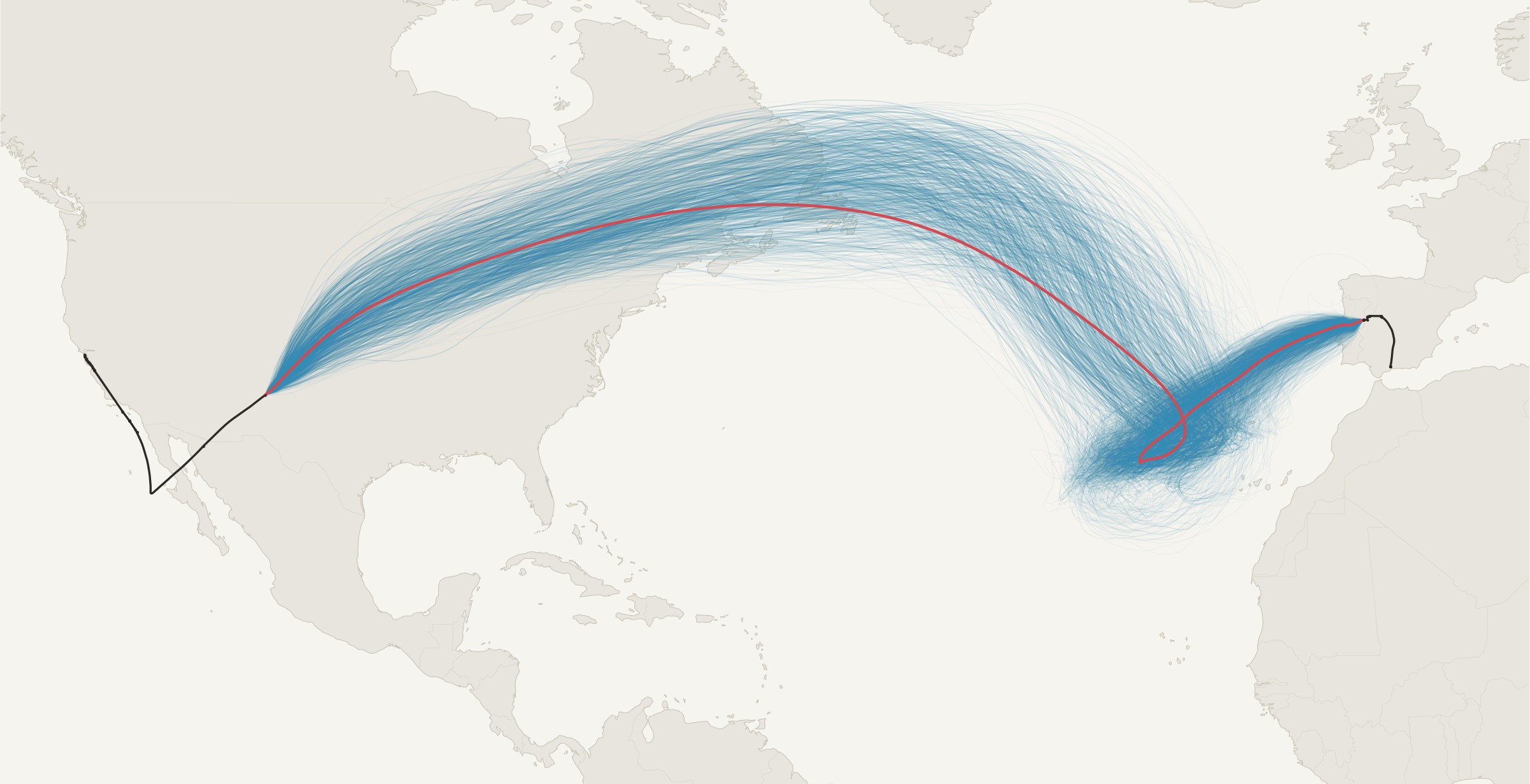
Knowing the path of the balloon is half the fun, so we want to have a way to reconstruct the route that it traveled between two points. The figure below shows the reconstructed path of Stratolink 3. It went eight days without sending a fix as it crossed from New Mexico to Spain.

Every distinct GPS fix Stratolink 3 sent, and the path the dashboard reconstructs through them. Over the Atlantic there are none for eight days.

What we know

For any gap, the problem is the same. We know where the balloon was at the two endpoints, and at what time. We also know roughly how high it was based on the readings from the pressure sensor. The balloon has no motor, so at a steady pressure it goes wherever the air at that pressure goes. Everything below follows from that.

Follow the winds

To find the path between the start and endpoints we need to follow the winds. At float altitude, winds rarely blow in a consistent direction and at constant speed and the balloon will follow in that path. We can use stratospheric wind data from weather models to give an estimate of how the winds transported the balloon.

A simulated balloon carried by the GFS winds alone from the New Mexico fix. When Stratolink 3 next reported from Spain, the simulated balloon was about 610 km away.

Unfortunately, wind data is not precisely measurable in the atmosphere, and these wind models only provide an approximation of the balloon’s path. As seen in the figure, naively tracing the wind field doesn’t result in the balloon reaching the right endpoint at the right time.

A little noise, a huge spread

So the winds from the model, and the balloon’s path by extension, may not match reality. How much can that matter? To test, we’ll simulate a set of balloons and give them slight deviations from the wind. We’ll move the wind’s direction by a few degrees, increase or decrease the wind speed by a little bit, or change the balloon’s height within the wind field. We’ll let them loose and see how close they end up.

500 simulated balloons run forward from the New Mexico fix with small errors in heading, speed and height (gray), around the path of the winds alone (black).

After simulating these balloons for eight days we see that the potential paths of the balloon stretch across the Atlantic, Europe and North Africa. The median balloon ends 3,590 km from where the balloon really was, and fewer than one in two hundred end within 300 km of it. The errors are small, but a balloon a few degrees off early on can end up on an entirely different path. Small differences grow until the possibilities span an ocean, which is also why weather forecasts give out after a week or so.

Arriving at the right place and time

Look closely at the end of that last figure, though. A handful of those balloons finish near the fix in Spain: six of the 500 end within 500 km of it, and the closest is 124 km away. Their paths are the interesting ones. They left the first fix when the balloon did, and they were close to the second fix at the moment the balloon was really there. What we want is a whole set of paths like that: ones that start at the first fix, follow the winds, and arrive at the second fix at the right time.

The same 500 simulated balloons, with the six that end within 500 km of the fix in Spain drawn along their whole route.

That changes the question. It isn’t where the balloon could have gone from the first fix. It’s which paths between the two fixes the winds make most probable.

Why not just run more balloons?

How can we find the most likely paths that satisfy both ends? The obvious answer is to simulate far more balloons and keep only the ones that arrive. The trouble is how few do. Two of these 500 ended within 300 km of the fix. To collect 2,000 paths like that we would need to simulate around half a million balloons, and 300 km still isn’t very close. Asking for 50 km would take something like 20 million. Nearly all of that work would go into balloons that end up over Norway or Libya.

So instead of aiming from one end, we start from both. One set of balloons starts at the first fix and moves forward in time. A second set starts at the second fix and moves backward in time, through the same winds run in reverse. That works because a balloon has no say in where it goes: if the wind carried it from one place to another, running the wind backward carries it back again. Each set only has to cover half the gap, and each is pinned to one of the two places we know the balloon was.

Meeting in the middle

Both sets get the same small errors as before: headings a few degrees off the wind, speeds a little fast or slow, heights that wander. For the eight-day gap each set has 8,000 balloons. A balloon that wanders out of the winds we’ve stored counts for less, and when a few balloons end up carrying most of the weight, the set is refreshed by dropping the weak ones and copying the strong ones, so the cloud never collapses onto a handful of them.

Balloons run forward from New Mexico (blue) and backward from Spain (red). They meet halfway through the gap, and the joined paths and the drawn line take their place.

Halfway through the gap the two clouds meet, and we need to join them up. Every forward balloon is paired with every backward balloon near it, and each pair gets a weight based on how well its two halves agree. We don’t just compare them at the midpoint. We compare them across a window either side of it, eight hours each way on the eight-day gap. Two halves that sit on top of each other for that whole stretch are very likely the same journey, so the pair gets a large weight. Two that run alongside each other but apart get a small one. Two that touch at the midpoint while heading in different directions pull apart within hours, so they get almost none. Inside the window, the two halves of a pair are blended into one continuous path.

How a pair is weighted: by how far apart its forward and backward halves are across the whole window, not just where they meet.

This is where meeting in the middle pays off. Pairing two clouds tries every combination of a forward half and a backward half for the cost of simulating just the two clouds. On Stratolink 3’s gap, 8,000 forward balloons times 8,000 backward ones is 64 million candidate paths, and about 600,000 of them carry meaningful weight. Every one of those starts on the first fix, ends on the second at the right time, and follows the winds in between. The dashboard keeps 2,000 of them, picked in proportion to their weights, and the whole reconstruction runs in under a minute.

Not every gap is eight days. Gaps under 20 minutes are joined with a straight line. Gaps from 20 minutes to six hours get a small version of the same idea: solve for the small speed and heading correction that makes a path driven by the wind land on the next fix, launch 200 simulated balloons from each fix, run the forward ones toward the far fix and the backward ones through time-reversed winds toward the near one, weight each by how close it lands, and average. Gaps of six hours and more, overnight gaps included, get the two clouds meeting in the middle. On Stratolink 3 that is 246 gaps of the first kind, 4 of the second and 4 of the third, and those last 4 hold 92% of the flight.

What a simulated balloon assumes

Each simulated balloon moves with the GFS wind at its own pressure, interpolated between the surrounding grid points, time slices and pressure levels, in 20-minute steps. Its heading offset and speed factor wander around zero with spreads of 12° and 15% and a memory of about 18 hours. Its pressure starts at the reading from its fix and wanders with an 8 hPa spread and a memory of about two days, around a line between the readings at the two ends of the gap.

Choosing one path

Now we have a set of candidate paths, each weighted by how plausible it is. The dashboard draws one line, so we need one path through them. We use their average position at each hour, which is our best single guess of where the balloon was at any moment.

The candidate paths across the eight-day gap, and the drawn line: their average position at each hour. The dots are where every path is at the hour the line has reached, lighter for paths that are behind and darker for those ahead.

Watch the dots as they come over Newfoundland. The paths don’t all move at the same speed, so at any hour they’re strung out along the route, the slow ones behind and the fast ones ahead. Average a set of points strung along a bend and you land on the inside of it, which is why the red line runs along the southern edge of the bundle across the top of the arc. It looks off-center, but it’s still the better guess. When we tested it, treating each path in turn as the true flight, the hourly average stayed closer to it than a line through the visual middle of the bundle.

Averages can mislead, though. If the paths split, say around a patch of slow air, the average of two routes runs between them, through places the balloon never was. So every two hours we compare how many paths lie within 300 km of the average with how many lie within 300 km of the center of the biggest bundle. If the average holds fewer than half as many, the routes have split, and the line follows the biggest bundle instead. On Stratolink 3 no gap splits, and the line moves by under 20 km when the whole job is rerun.

The line is still the center of the routes the winds allow, not a measurement. In the middle of the eight-day gap, 90% of the paths fall within 500 to 800 km of it. It’s our best single guess through a corridor that wide, and showing that corridor on the dashboard, not just the line, is the next thing I want to build.

Putting it together

That’s the whole method. To draw a line across a gap:

Start from what we know: where the balloon was at each end of the gap, when, and roughly how high it was flying.
Let a cloud of simulated balloons ride the model winds forward from the first fix, and another ride them backward from the second, each with small errors of its own.
Where the two clouds meet, pair them up and weight each pair by how well its two halves agree.
Draw the line through the densest part of the paths that result.

Every path we keep starts on one fix, ends on the other at the right time, and follows the winds in between. On their own, the winds got the shape of Stratolink 3’s crossing but missed Spain by hundreds of kilometers, and a cloud aimed from one end spread across an ocean. Working from both ends turns eight days of silence over the Atlantic into a route, in under a minute.

Where it goes next

The forward forecast is the same integration pointed at the future, with one change. Instead of perturbing a single wind field, each path rides a different model run. NOAA’s Global Ensemble Forecast System, GEFS, publishes 31 members, each started from slightly different initial conditions, and its machine-learning counterpart AIGEFS publishes another 31.² We cut a tube for every member and integrate the balloon from the last fix through each one, which gives 62 paths that disagree exactly as much as the weather models do.

The line the dashboard draws is the per-hour median of the members, and the forecast ends at the first hour where the 75th-percentile distance of the members from that median passes 2,000 km. Past that point the members are spread across a continent and the median isn’t predicting anything. From Stratolink 3’s last fix near Málaga on May 29, the members ran east across the Mediterranean, Asia and the Pacific, and their spread crossed 2,000 km on June 9, ten and a half days out, over Utah.

The 62 members from the last fix, GEFS in blue and AIGEFS in red, with the spread that decides where the forecast stops.

A balloon that stops reporting for good turns the stretch from its last fix to now into a forecast as well, and the dashboard draws it as one. Stratolink 3 never sent another position; the route at the top of Teddy’s June post came from an earlier experiment with this machinery, pushed on for weeks toward a guessed endpoint. The forecast now stops when the models stop agreeing, which is the honest place to stop.

The positions we did receive, and the line through them, are on Stratolink 3’s flight. Shepherd’s Baja Run covers the first two days, and Teddy’s Looking for Stratolink 3 picks up after the last packet.

Appendix

The details behind the method: where the winds come from, how we check a reconstruction, how much the answer depends on the jitter, and how it all runs.

Where the winds come from

The winds come from GFS, which runs four times a day. NOAA puts every run in a public S3 bucket with an index of the byte range of each field, so we can fetch just the wind fields we need, for free and without an API key.¹ For the reconstruction we read four pressure levels around the balloon’s float, 200, 250, 300 and 350 hPa, from the model’s analyses every three hours; for the forecast, the latest cycle’s hourly winds blended to the float pressure.

Each field is the whole globe, a million grid points, so the winds a balloon needs are cut into a tube: a stack of three-hour slices, each a box at full 0.25° resolution. Around a short gap the box sits on the line between the two fixes. Inside a long gap it follows the winds: before the box is cut, a small pilot cloud of simulated balloons is run forward from the fix before the gap and backward from the fix after it, and each box is sized to hold those clouds over the six hours it is read. That matters, because a long gap rarely runs along the line between its fixes. The winds took Stratolink 3 to the middle of the Atlantic in two days and then held it for four in a slow loop west of the Azores; a tube laid along the straight line to Spain would have been somewhere else entirely by the second day. Around every box the cube also keeps the wind at a coarser 1.5° over most of the hemisphere, so a balloon that wanders out of the box still rides real winds. For Stratolink 3 the reconstruction cube is about 22 MB and the hourly forecast cube 1.8 MB.

Riding the tube: each three-hour slice’s box moving along the flight with the 0.25° winds inside it and the coarser 1.5° winds around it (pale), the clouds of simulated balloons from New Mexico (blue) and Spain (red), and the paths that join them (black). The forward cloud doesn’t know where Spain is, so it spreads well past the box onto the coarser winds; the joined paths stay inside it.

What the box resolves: a 3° square around the balloon at each field’s real density, and the difference between them. Near the balloon the two typically differ by 1 to 2 m/s, small, but steady over days, and the box also carries the four pressure levels the coarse field doesn’t.

Checking it

The first thing to check on any reconstruction is whether the balloon behaves like a balloon. For every step of every path, we measure the angle between the direction it moved and the wind at that place and time. If the simulated balloons could fly across the flow, this is where it would show. On Stratolink 3’s eight-day gap, nine steps in ten are within 20° of the wind, about the same as the forecast ensemble shows, and the paths move at the wind’s speed.

The other checks are about stability: how closely the forward and backward clouds meet, and how far the drawn line moves when the whole thing is rerun. On the eight-day gap the clouds meet within about 45 km of each other and the line moves by about 10 km. If the winds can’t connect the two ends of a gap at all, the reconstruction says so instead of drawing a line. And the path of the winds alone, from earlier, is a check too. With no randomness at all, the GFS winds take the same route the joined paths do, up the jet over Newfoundland, around the loop near the Azores and into Iberia from the southwest, and run backward from Spain they trace it too. The joined paths don’t invent a route to connect the fixes. They take the one the winds already offer and bend it by small amounts until it lands on both ends. The eight-day gap is explained by the winds at the balloon’s own altitude.

How much jitter?

The small errors each simulated balloon carries, a heading spread of ±12°, a speed spread of ±15% and a height spread of ±8 hPa, aren’t precise measurements. They came from the few clean pairs of GPS fixes Stratolink 3 gave us. So we checked how much the answer depends on them by rerunning the eight-day gap 125 times, across five values of each.

The eight-day gap at 25 heading and speed settings, each a full run with 8,000 balloons each way. Select a cell to map its paths and line against today’s.

The line holds up. Across heading spreads of ±8 to ±18° and speed spreads of ±5 to ±15%, at any height spread, it moves a typical 25 to 85 km from today’s, where just rerunning today’s settings moves it about 13 km. Only at the edges of the grid, ±24° of heading or ±22% of speed and up, does it move by hundreds of kilometers. What does change is the corridor. Speed spread sets how wide the plausible routes are, from about 500 km mid-gap at ±5% to more than 1,200 km at ±30%, and from ±22% up the paths split into separate routes. Height spread barely matters.

Is there a right setting? One way to ask the data is to score each setting by how likely the forward and backward clouds are to meet. That score keeps rising as the heading spread shrinks, and peaks around ±5% of speed. GFS seems to have the wind’s direction right, and a little speed variation is what lets a balloon’s timing work out. By that measure today’s settings are on the generous side. But the score comes from a single gap, and it can’t tell us whether the corridor is realistically wide. Pinning these numbers down will take flights with long, well-tracked stretches we can hide and reconstruct.

The plumbing

Four runs a day while a balloon is flying; nothing runs when the fleet is quiet.

All of this runs on a GitHub Actions runner, four times a day. A run starts by deciding which balloons need work. A balloon whose last fix is more than 15 days old and whose stored forecast already ends at its divergence point cannot change, so it is skipped, and when the fleet is quiet the run plans nothing, downloads nothing and exits. When a balloon is flying, the runner pulls the wind fields it needs from NOAA’s bucket by byte range, builds the two cubes plus a tube per ensemble member, runs the reconstruction and the forecast, and writes one JSON file per balloon, about half a megabyte, to Vercel Blob. The dashboard reads that file and draws.

Each reconstructed gap is cached by a hash of its two fixes, the pressure level and the method version, so a rerun only recomputes the gaps that changed. For Stratolink 3 the whole compute, reconstruction and forecast together, takes under a minute on the runner. The ingest takes longer, and almost all of it is waiting on S3 for the member cubes; when a few members don’t arrive inside the step’s time budget, the forecast runs on the ones that did.

Where the code is

Everything is in the Stratolink repository, under web/. The ingest is scripts/gfs_ingest.py, with gefs_ingest.py and aigefs_ingest.py for the ensemble members. The cube format and wind sampling are in lib/wind/windCube.ts, the short and medium gaps in lib/wind/pathReconstruction.ts, the long-gap filters and the drawn line in lib/wind/pathReconstructionLongGap.ts, and the forecast in lib/wind/monteCarloForecast.ts. The schedule is .github/workflows/gfs-ingest.yml.

Data sources

NOAA GFS on the AWS Open Data Registry: noaa-gfs-bdp-pds, 0.25° GRIB2 with a byte-range index for every field.
NOAA GEFS: noaa-gefs-pds, 31 members at 0.5°. AIGEFS members come from the noaa-nws-graphcastgfs-pds bucket at 0.25°.
Coastlines and borders in the figures are from Natural Earth.